A first model
In this tutorial, we will fit an example SEM with our package. The example we are using is from the lavaan tutorial, so it may be familiar. It looks like this:
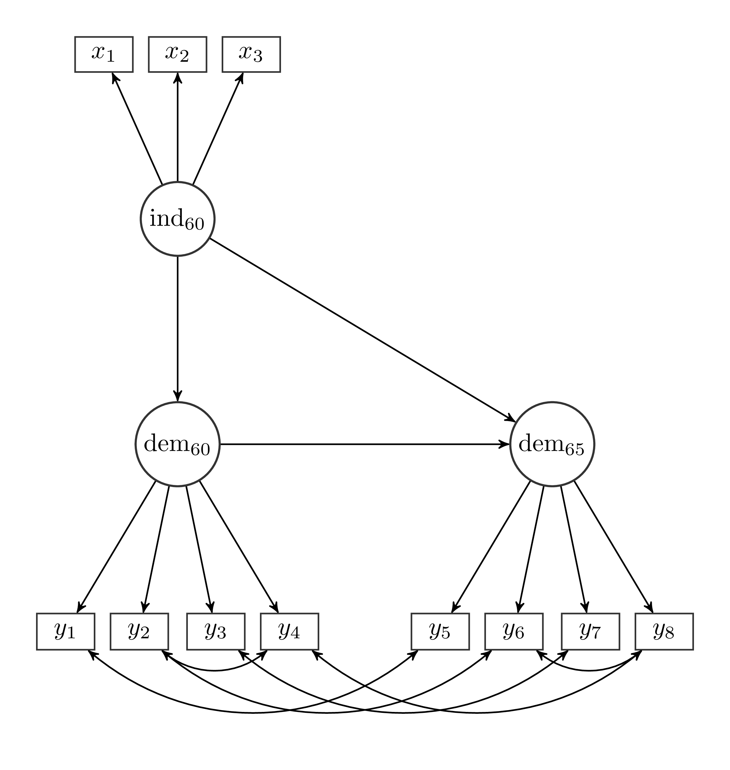
We assume the StructuralEquationModels package is already installed. To use it in the current session, we run
using StructuralEquationModelsWe then first define the graph of our model in a syntax which is similar to the R-package lavaan:
obs_vars = [:x1, :x2, :x3, :y1, :y2, :y3, :y4, :y5, :y6, :y7, :y8]
lat_vars = [:ind60, :dem60, :dem65]

graph = @StenoGraph begin

    # loadings
    ind60 → fixed(1)*x1 + x2 + x3
    dem60 → fixed(1)*y1 + y2 + y3 + y4
    dem65 → fixed(1)*y5 + y6 + y7 + y8

    # latent regressions
    ind60 → dem60
    dem60 → dem65
    ind60 → dem65

    # variances
    _(obs_vars) ↔ _(obs_vars)
    _(lat_vars) ↔ _(lat_vars)

    # covariances
    y1 ↔ y5
    y2 ↔ y4 + y6
    y3 ↔ y7
    y8 ↔ y4 + y6

endWhen executing the code from this tutorial the first time in a fresh julia session, you may wonder that it takes quite some time. This is not because the implementation is slow, but because the functions are compiled the first time you use them. Try rerunning the example a second time - you will see that all function executions after the first one are quite fast.
We then use this graph to define a ParameterTable object
partable = ParameterTable(
    graph,
    latent_vars = lat_vars,
    observed_vars = obs_vars)
-------- ---------- -------- ------- ------------- --------- ---------- -------
from relation to free value_fixed start estimate lab ⋯
Symbol Symbol Symbol Bool Float64 Float64 Float64 Symb ⋯
-------- ---------- -------- ------- ------------- --------- ---------- -------
ind60 → x1 false 1.0 con ⋯
ind60 → x2 true θ ⋯
ind60 → x3 true θ ⋯
dem60 → y1 false 1.0 con ⋯
dem60 → y2 true θ ⋯
dem60 → y3 true θ ⋯
dem60 → y4 true θ ⋯
dem65 → y5 false 1.0 con ⋯
dem65 → y6 true θ ⋯
dem65 → y7 true θ ⋯
dem65 → y8 true θ ⋯
ind60 → dem60 true θ ⋯
dem60 → dem65 true θ_ ⋯
ind60 → dem65 true θ_ ⋯
x1 ↔ x1 true θ_ ⋯
⋮ ⋮ ⋮ ⋮ ⋮ ⋮ ⋮ ⋱
-------- ---------- -------- ------- ------------- --------- ---------- -------
1 column and 19 rows omitted
Latent Variables: [:ind60, :dem60, :dem65]
Observed Variables: [:x1, :x2, :x3, :y1, :y2, :y3, :y4, :y5, :y6, :y7, :y8]
load the example data
data = example_data("political_democracy")and specify our model as
model = Sem(
    specification = partable,
    data = data
)
Structural Equation Model- Loss Functions
> SemML
- observed: SemObservedData
- implied: RAM
We can now fit the model via
model_fit = fit(model)Fitted Structural Equation Model
===============================================
--------------------- Model -------------------
Structural Equation Model- Loss Functions
  > SemML
    - observed:    SemObservedData
    - implied:     RAM
------------- Optimization result -------------
engine: Optim
* Status: success
* Candidate solution
Final objective value: 2.120543e+01
* Found with
Algorithm: L-BFGS
* Convergence measures
|x - x'| = 3.77e-05 ≰ 1.5e-08
|x - x'|/|x'| = 5.05e-06 ≰ 0.0e+00
|f(x) - f(x')| = 1.28e-09 ≰ 0.0e+00
|f(x) - f(x')|/|f(x')| = 6.04e-11 ≤ 1.0e-10
|g(x)| = 1.21e-04 ≰ 1.0e-08
* Work counters
Seconds run: 0 (vs limit Inf)
Iterations: 174
f(x) calls: 226
∇f(x) calls: 226
∇f(x)ᵀv calls: 0
and compute fit measures as
fit_measures(model_fit)Dict{Symbol, Real} with 8 entries:
:AIC => 3168.66
:BIC => 3240.5
:CFI => 0.99607
:χ² => 37.6169
:dof => 35.0
:p_value => 0.350263
:nparams => 31
:RMSEA => 0.0317865We can also get a bit more information about the fitted model via the details() function:
details(model_fit)
Fitted Structural Equation Model

--------------------------------- Properties ---------------------------------

Optimization engine:         Optim
Optimization algorithm:      L-BFGS
Convergence:                 [:f_converged]
No. iterations/evaluations:  174

Number of parameters:        31
Number of data samples:      75

----------------------------------- Model ------------------------------------

Structural Equation Model (Sem)
- 31 parameters
- Loss Functions:
  - SemML (75 samples, 11 observed, 3 latent variables) w=1
To investigate the parameter estimates, we can update our partable object to contain the new estimates:
update_estimate!(partable, model_fit) -------- ---------- -------- ------- ------------- --------- ----------- ------
from relation to free value_fixed start estimate la ⋯
Symbol Symbol Symbol Bool Float64 Float64 Float64 Sym ⋯
-------- ---------- -------- ------- ------------- --------- ----------- ------
ind60 → x1 false 1.0 1.0 co ⋯
ind60 → x2 true 2.18038 ⋯
ind60 → x3 true 1.8185 ⋯
dem60 → y1 false 1.0 1.0 co ⋯
dem60 → y2 true 1.25675 ⋯
dem60 → y3 true 1.05773 ⋯
dem60 → y4 true 1.26478 ⋯
dem65 → y5 false 1.0 1.0 co ⋯
dem65 → y6 true 1.18569 ⋯
dem65 → y7 true 1.27952 ⋯
dem65 → y8 true 1.26595 ⋯
ind60 → dem60 true 1.48294 ⋯
dem60 → dem65 true 0.837327 θ ⋯
ind60 → dem65 true 0.572397 θ ⋯
x1 ↔ x1 true 0.0826512 θ ⋯
⋮ ⋮ ⋮ ⋮ ⋮ ⋮ ⋮ ⋱
-------- ---------- -------- ------- ------------- --------- ----------- ------
1 column and 19 rows omitted
Latent Variables: [:ind60, :dem60, :dem65]
Observed Variables: [:x1, :x2, :x3, :y1, :y2, :y3, :y4, :y5, :y6, :y7, :y8]
and investigate the solution with
details(partable)
---------------------------------- Variables ---------------------------------

Latent variables:    ind60 dem60 dem65
Observed variables:  x1 x2 x3 y1 y2 y3 y4 y5 y6 y7 y8

---------------------------- Parameter Estimates -----------------------------

Loadings:

ind60


  to   estimate   value_fixed   start   free   from    label   relation

  x1   1.0        1.0                   0.0    ind60   const   →
  x2   2.18                             1.0    ind60   θ_1     →
  x3   1.82                             1.0    ind60   θ_2     →


dem60


  to   estimate   value_fixed   start   free   from    label   relation

  y1   1.0        1.0                   0.0    dem60   const   →
  y2   1.26                             1.0    dem60   θ_3     →
  y3   1.06                             1.0    dem60   θ_4     →
  y4   1.26                             1.0    dem60   θ_5     →


dem65


  to   estimate   value_fixed   start   free   from    label   relation

  y5   1.0        1.0                   0.0    dem65   const   →
  y6   1.19                             1.0    dem65   θ_6     →
  y7   1.28                             1.0    dem65   θ_7     →
  y8   1.27                             1.0    dem65   θ_8     →


Directed Effects:


  from        to      estimate   value_fixed   start   free   label

  ind60   →   dem60   1.48                             1.0    θ_9
  dem60   →   dem65   0.84                             1.0    θ_10
  ind60   →   dem65   0.57                             1.0    θ_11


Variances:


  from        to      estimate   value_fixed   start   free   label

  x1      ↔   x1      0.08                             1.0    θ_12
  x2      ↔   x2      0.12                             1.0    θ_13
  x3      ↔   x3      0.47                             1.0    θ_14
  y1      ↔   y1      1.92                             1.0    θ_15
  y2      ↔   y2      7.47                             1.0    θ_16
  y3      ↔   y3      5.14                             1.0    θ_17
  y4      ↔   y4      3.19                             1.0    θ_18
  y5      ↔   y5      2.38                             1.0    θ_19
  y6      ↔   y6      5.02                             1.0    θ_20
  y7      ↔   y7      3.48                             1.0    θ_21
  y8      ↔   y8      3.3                              1.0    θ_22
  ind60   ↔   ind60   0.45                             1.0    θ_23
  dem60   ↔   dem60   4.01                             1.0    θ_24
  dem65   ↔   dem65   0.17                             1.0    θ_25


Covariances:


  from       to   estimate   value_fixed   start   free   label

  y1     ↔   y5   0.63                             1.0    θ_26
  y2     ↔   y4   1.33                             1.0    θ_27
  y2     ↔   y6   2.18                             1.0    θ_28
  y3     ↔   y7   0.81                             1.0    θ_29
  y8     ↔   y4   0.35                             1.0    θ_30
  y8     ↔   y6   1.37                             1.0    θ_31
Congratulations, you fitted and inspected your very first model! We recommend continuing with Our Concept of a Structural Equation Model.